Introduction to Data Management for Researchers

Great Court, The University of Queensland

Introduction

This tutorial introduces fundamental data management practices for researchers working with language data. Good data management is not a bureaucratic chore — it is what separates a project that can be reproduced, shared, and built upon from one that exists only in a single person’s memory.

What you will learn

Learning Objectives

By the end of this tutorial, you will be able to:

• explain why data management matters for reproducible research
• create a consistent, scalable folder structure for research projects
• apply effective file naming conventions
• choose appropriate file formats for long-term data preservation
• write useful metadata and README documentation
• apply the 3-2-1 backup rule to protect your data
• use basic version control with Git in RStudio

Citation

Martin Schweinberger. 2026. Introduction to Data Management for Researchers. The Language Technology and Data Analysis Laboratory (LADAL), The University of Queensland, Australia. url: https://ladal.edu.au/tutorials/datamanagement/datamanagement.html (Version 3.1.1). doi: 10.5281/zenodo.19424860.

Preparation and session set up

This tutorial requires the checkdown package for the interactive exercises. Install it if you have not already done so.

install.packages("checkdown")

library(checkdown)

---

Why Data Management Matters

Researchers routinely underestimate how much time poor data management costs them. A widely cited study found that researchers spend around 30% of their time simply searching for files they know they have somewhere (Tenopir et al. 2011). Multiplied across a career, that is an enormous loss of productive time — for something that good organisation can almost entirely prevent.

Beyond individual efficiency, data management underpins the credibility of science itself. More than 70% of researchers have been unable to reproduce another scientist’s results, and poor data practices are a major contributing factor (Baker 2016). When data are well organised, well documented, and stored safely, your findings can be verified, your analyses can be reused, and your work can contribute to the cumulative knowledge of the field.

The investment pays off quickly

Setting up good data management takes roughly 5–10 hours upfront, plus around 30 minutes per week of maintenance. In return, most researchers save well over 200 hours per year that would otherwise be spent searching for files, re-creating lost work, or untangling confusing folder structures. More importantly, you will be in a position to share your data, respond to reviewer requests, and meet the open data requirements of journals and funders.

Section overview

This section introduces the core motivation for data management. The sections that follow cover the practical skills: folder organisation, file naming, data formats, metadata, backups, and version control.

Q1. A colleague tells you they lost a week of analysis because they accidentally overwrote a processed data file with an uncleaned version. Which data management practice would have prevented this?

Saving the file with a longer, more descriptive name
Emailing a copy of the file to themselves before editing
Keeping raw data in a separate, read-only folder and only ever working with copies in a processed/ subfolder
Using a newer version of R

---

Folder Structure and File Organisation

Section overview

This section covers how to organise your project files in a way that is logical, scalable, and self-explanatory — both to collaborators and to your future self.

A standard project folder structure

The single most impactful data management decision you can make is to adopt a consistent folder structure for every project. Consistency means that anyone — including you six months from now — can navigate any of your projects immediately without having to remember how you organised that particular one.

The template below works well for most research projects in linguistics and the humanities. The numbered prefixes ensure folders sort in logical order regardless of the operating system.

ProjectName_YYYY/
├── README.md                     ← Read this first
├── 00_admin/
│   ├── ethics/
│   └── funding/
├── 01_data/
│   ├── raw/                      ← NEVER EDIT — original files only
│   ├── processed/                ← Working copies
│   └── metadata/                 ← Codebooks, data dictionaries
├── 02_scripts/
│   ├── 01_data_cleaning.R
│   ├── 02_analysis.R
│   └── 03_visualisations.R
├── 03_outputs/
│   ├── figures/
│   └── tables/
├── 04_manuscript/
│   ├── drafts/
│   └── submitted/
└── 05_archive/

A few principles underlie this structure. First, raw data lives in its own protected folder and is never touched after collection. Second, scripts are numbered so they can be run in order, making it clear how to reproduce the analysis from scratch. Third, outputs are separated from inputs so it is always obvious what was generated and what was provided.

Every project needs a README

A README file at the top level of every project folder is the single most useful piece of documentation you can write. It should explain what the project is, who is responsible for it, what each folder contains, how to reproduce the analysis, and where to find the data. Think of it as the instructions a new collaborator would need to get up to speed in an afternoon. See the documentation section below for a README template.

File naming conventions

File names are your first layer of documentation. A good file name tells you the date the file was created, what project it belongs to, what it contains, and what version it is — without opening it.

The recommended format is:

YYYY-MM-DD_project_description_version.extension

The ISO date format (year first) is essential because it sorts chronologically in any file browser. Using underscores instead of spaces matters because spaces break file paths in code. Version numbers prevent the all-too-common final_FINAL_USE_THIS_ONE.docx problem.

Examples of bad vs. good file names

❌  final.docx
❌  data.csv
❌  New Document (2).docx
❌  analysis final FINAL reviewed.R

✓  2026-03-15_surveyA_demographics_v1.csv
✓  2026-03-20_surveyA_cleaned_v2.csv
✓  2026-04-01_manuscript_draft_v3.docx
✓  01_data_cleaning.R

For analysis scripts, a simpler numbered prefix is often better than dates, since scripts tend to be run in a fixed order rather than indexed by date.

Q2. You are organising a corpus of historical letters collected in January 2026, cleaned in February, and used in a final analysis in March. Which set of file names follows best practice?

2026-01-10_letters_raw.txt / 2026-02-03_letters_cleaned.txt / 2026-03-15_letters_final_analysis.csv
Jan letters / Feb cleaned / Mar analysis final.csv
letters.txt / letters_clean.txt / letters_done.csv
data_v1.txt / data_v2.txt / data_final.csv

---

Data Formats

Section overview

Choosing the right file format affects whether your data will be readable in 10 or 20 years, how easily it can be shared, and whether it can be opened without proprietary software.

Choosing formats for long-term preservation

Not all file formats are equally suitable for research data. Proprietary formats (.xlsx, .docx, .sav) depend on specific software that may not be available to collaborators or in the future. Open, plain-text formats are preferable for data that needs to be shared or preserved.

Recommended file formats for research data preservation

Data type	Preferred format	Why
Tabular data	.csv	Plain text, universally readable, no software dependency
Text corpora	.txt (UTF-8)	Plain text, durable, portable
Annotated text	.xml, .conllu	Open standards, tool-independent
Audio recordings	.wav, .flac	Uncompressed / losslessly compressed
Images	.tiff, .png	Uncompressed or lossless
Documents	.pdf/A	Archival PDF standard
Code	.R, .py, .qmd	Plain text, version-controllable

For working files (files you edit every day), proprietary formats like .xlsx and .docx are fine. The key rule is that when you reach a milestone — data collection complete, analysis finalised, paper submitted — you save a copy in an open format for archiving and sharing.

Avoid format dependency

Never store your only copy of a dataset in a format that requires a specific paid application to open. If SPSS, NVivo, or a particular version of Excel becomes unavailable, your data becomes inaccessible. Always export a plain-text copy (.csv, .txt) alongside any proprietary working file.

Text encoding

For text data specifically, encoding matters enormously. Unicode (UTF-8) is the standard for modern text data and handles virtually every writing system. Always save text files as UTF-8, and always check the encoding when loading text data in R.

# Always specify encoding when reading text files
corpus_text <- readLines("data/raw/letters.txt", encoding = "UTF-8")

# Or when reading tabular data
survey_data <- read.csv("data/raw/survey.csv", fileEncoding = "UTF-8")

Q3. A colleague gives you a dataset as a .sav file (SPSS format). What is the best approach?

Open it in R using the haven package, inspect it, then export a .csv copy as the archival version
Rename the file to .csv — renaming changes the format
It is fine as-is; .sav is an industry standard
Only use it if you have SPSS installed

---

Metadata and Documentation

Section overview

Metadata is data about your data. Without it, even a perfectly organised folder of well-named files can be opaque to anyone who did not create them — including yourself six months later.

README files

A README is a plain-text or Markdown file that lives at the top of a project folder and explains everything a new person would need to understand and use the project. The template below covers the most important sections:

# Project Title: [Your Project Name]

## Overview
[2–3 sentence description of what this project is about]

**Principal Investigator**: [Name] ([email])
**Start Date**: YYYY-MM-DD
**Funding**: [Source, Grant #]
**Ethics Approval**: [Number]

## Research Question
[What specific question(s) does this project address?]

## Folder Structure
- `00_admin/`: Ethics approvals, funding documents
- `01_data/raw/`: Original data files — DO NOT EDIT
- `01_data/processed/`: Cleaned and processed versions
- `01_data/metadata/`: Codebooks and data dictionaries
- `02_scripts/`: Analysis scripts (run in numbered order)
- `03_outputs/`: Generated figures and tables
- `04_manuscript/`: Paper drafts and submissions

## How to Reproduce the Analysis
1. Open `ProjectName.Rproj` in RStudio
2. Run `renv::restore()` to install all required packages
3. Run scripts in order: 01 → 02 → 03
4. Outputs will appear in `03_outputs/`

## Data Description
- **Source**: [Where data came from]
- **Collection period**: [Dates]
- **Sample size**: N = [number]
- **Key variables**: [Brief description]

## Software
- R version 4.4.x
- Key packages: tidyverse, lme4 (see renv.lock for full list)

## Contact
[Name], [email] — Last updated: YYYY-MM-DD

Codebooks and data dictionaries

For any dataset, every variable should be documented in a codebook that explains what the variable is, what type it is, what its values mean, and how missing data are coded. Without a codebook, a dataset of numbers is nearly uninterpretable.

Example data dictionary for a survey dataset

Variable	Description	Type	Values / Range	Missing
participant_id	Unique participant code	Character	P001–P150	None
age	Age in years at time of data collection	Integer	18–75	-99 = refused
gender	Self-reported gender	Categorical	1 = Woman; 2 = Man; 3 = Non-binary; 4 = Self-describe; 5 = Prefer not to say	NA
test_score	Score on cognitive task (% correct)	Numeric	0–100	-99 = incomplete

The codebook should be stored in 01_data/metadata/ alongside the dataset it describes, so they always travel together.

Processing logs

Every transformation applied to your data should be recorded. The most reliable way to do this is to use R scripts that document the transformations in code — a script that cleans your data is a processing log. But a separate plain-text log is also valuable for recording decisions made outside of code (e.g. “excluded participant P047 because they reported not reading the instructions”):

# Data Processing Log

## 2026-02-01 — Initial cleaning
Script: 01_data_cleaning.R
Changes:
  - Removed 15 duplicate rows (same participant_id, identical responses)
  - Converted date format from DD/MM/YYYY to ISO YYYY-MM-DD
  - Recoded -999 to NA for all missing value fields
  - Excluded 3 test responses (participant_id = "TEST")
Result: N reduced from 150 to 132

## 2026-02-05 — Variable creation
Script: 02_create_variables.R
Changes:
  - Created age_group (18–25, 26–40, 41–60, 61+)
  - Created composite_score (mean of items Q1–Q10)
  - Reverse-coded items Q5, Q8, Q12
Result: 3 new variables added

Q4. You return to a dataset after eight months away. The folder contains files named data_v1.csv, data_v2.csv, data_FINAL.csv, and data_clean.csv, with no README and no processing log. What would have most helped you know which file to use?

Deleting all files except the final one at the end of the project
Remembering which file was most recent
Using a larger hard drive so more versions can be stored
A README explaining the folder structure and a processing log recording what was done to each version

---

Data Safety and Backups

Section overview

Backups protect against hardware failure, accidental deletion, theft, and disaster. The 3-2-1 rule is the research community’s standard for reliable data protection.

The 3-2-1 backup rule

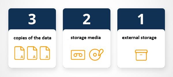
The 3-2-1 rule is simple and non-negotiable:

• 3 copies of your data (1 primary working copy + 2 backups)
• 2 different storage media (e.g. local drive + external drive)
• 1 copy stored offsite (cloud storage or an external drive kept at a different physical location)

This combination protects against the most common failure scenarios. A local hard drive failure destroys the working copy, but the external drive survives. A fire or flood destroys both local copies, but the offsite copy survives.

For most researchers, a practical implementation is:

• Working copy: laptop or desktop
• Backup 1: external hard drive, updated weekly
• Backup 2: cloud storage (continuous automatic sync)

Sensitive data and cloud storage

Standard consumer cloud services (Google Drive, Dropbox, iCloud, personal OneDrive) are not approved for storing sensitive research data — including identifiable participant information, health data, or legally confidential material. For sensitive data, use your institution’s approved research data storage (at UQ, this is the Research Data Manager — RDM). Encrypted external drives are a suitable alternative for local backup.

Automation is your friend

Manual backups are better than nothing, but automated backups are much more reliable because they do not depend on you remembering. The most practical approach combines two layers:

• Continuous cloud sync: Turn on automatic sync in OneDrive or Google Drive for non-sensitive working files. Changes are backed up in seconds.
• Scheduled local backup: Use Time Machine (macOS) or Windows Backup to back up to an external drive hourly or daily. Set this up once and let it run.

For sensitive data that cannot go to the cloud, a monthly manual backup to an encrypted external drive, combined with your institution’s RDM, is a solid approach.

Q5. A fire destroys a researcher’s office, including their laptop and the external hard drive sitting on their desk. Their only other copy was in a Dropbox folder on the same laptop. How many copies of the data do they now have?

One — the Dropbox cloud copy survived, but the laptop and desk drive were both destroyed
Zero — all copies were destroyed
Three — they had three copies as required by the 3-2-1 rule
Two — the laptop hard drive and the Dropbox copy both survived

---

Version Control with Git

Section overview

Version control is a system for tracking changes to files over time, so you can see exactly what changed, when, and why — and revert to any previous state if needed. Git is the most widely used version control system in research and software development.

Why version control?

Without version control, file versioning tends to look like this:

manuscript_draft.docx
manuscript_draft_final.docx
manuscript_draft_final_FINAL.docx
manuscript_draft_final_FINAL_reviewed.docx
manuscript_USE_THIS_ONE.docx

With Git, there is a single file containing the current version, plus a complete history of every change ever made to it — including who made the change, when, and a short message explaining why. You can revert to any previous state at any time.

Core Git concepts

Repository (repo): a project folder tracked by Git — it contains all your files plus their complete history.

Commit: a saved snapshot of the project at a specific moment in time, with a short message describing what changed.

Push: uploading your local commits to a remote repository (e.g. GitHub).

Pull: downloading changes from a remote repository to your local machine.

Branch: a parallel version of the project used to develop a new feature or experiment without affecting the main version.

Using Git in RStudio

RStudio has built-in Git support, meaning you can do everything through a graphical interface without using the command line.

Setup (once per project):

1. Create a new project: File → New Project → New Directory
2. Check the box “Create a git repository”
3. To connect to GitHub: Tools → Shell and follow the GitHub authentication steps

Daily workflow:

1. Pull at the start of each session to get any changes from collaborators
2. Make changes to your files
3. Open the Git pane (top-right in RStudio)
4. Stage changed files by ticking the checkbox next to them
5. Commit with a short, descriptive message
6. Push to GitHub

For those who prefer the command line, the equivalent commands are:

# Stage all changed files
git add .

# Commit with a message
git commit -m "Add descriptive statistics analysis"

# Push to GitHub
git push origin main

Writing good commit messages

A commit message should complete the sentence “If applied, this commit will…”. Use the imperative mood and be specific:

✓  Add demographic variables to cleaned dataset
✓  Fix encoding error in corpus loading script
✓  Remove outliers beyond ±3 SD from test_score
✓  Update regression model to include gender covariate

❌  stuff
❌  changes
❌  update
❌  final version (really this time)

Good commit messages make it possible to understand the history of a project at a glance, which is invaluable when something breaks and you need to find the last version that worked.

Not everything belongs in Git

Git is designed for plain-text files: R scripts, Markdown documents, CSV data, and similar. It works poorly with large binary files (audio recordings, large datasets, images), which should be stored in cloud storage or a data repository instead. For large file support in Git, there is Git Large File Storage (LFS), but for most research projects the simpler rule is: code and documentation go in Git; large data files go in the cloud or a data repository.

Q6. After running your analysis, you discover that a change you made three commits ago introduced a bug that affected your results. What Git feature allows you to recover the working version from before that change?

The commit history — you can check out or revert to any earlier commit to restore the files as they were at that point
The branch — you can delete the current branch and start a new one
Git cannot help here; you would need to find an older backup
The README — it documents what the code does so you can rewrite it

---

Data Sharing and FAIR Principles

Section overview

Sharing data is increasingly required by journals and funders, and it benefits science by enabling verification and reuse. This section covers the FAIR principles and the practical steps for sharing your data responsibly.

The FAIR principles

The FAIR principles define what it means for research data to be well-managed and shareable:

• Findable: data has a persistent identifier (such as a DOI), rich metadata, and is indexed in a searchable resource
• Accessible: data can be retrieved via its identifier; metadata remains accessible even if the data itself is restricted
• Interoperable: data uses standard, open formats and standard vocabularies so it can be combined with other data
• Reusable: data is well documented, has a clear license, and meets community standards

FAIR does not mean unrestricted open access — it means that the data is managed well enough that authorised users can find and use it. Sensitive data can still be FAIR if it is documented, stored in an approved repository, and accessible under appropriate conditions.

Persistent identifiers

A Digital Object Identifier (DOI) is a permanent link to a research output (paper, dataset, or code). Unlike a regular URL, a DOI is maintained permanently even if the underlying web address changes. Sharing your data with a DOI means the link will always work, your data will be citable, and usage metrics can be tracked.

For data: repositories like Zenodo, OSF, figshare, and TROLLing (linguistics-specific) all issue DOIs automatically. At UQ, the Research Data Manager (RDM) connects to UQ eSpace to issue DOIs for datasets.

For code: connecting your GitHub repository to Zenodo allows you to issue a DOI for each software release.

What to share

At minimum, a shareable data package should include the final analysed dataset (deidentified if necessary), the analysis code, a README, and a codebook or data dictionary. A complete package would also include the raw data (if shareable), all processing scripts, and ideally the computing environment specification (renv.lock in R).

Before sharing, work through this checklist:

• Ethics approval permits data sharing
• Participants consented to data being shared
• Data is deidentified (if required)
• All variables are labelled and documented in a codebook
• Missing data is coded consistently and documented
• A README file is included
• Analysis code is included and tested
• An appropriate license is applied (CC-BY 4.0 is standard for open data)

---

Quick Reference

File naming template

YYYY-MM-DD_project_description_version.extension

Example: 2026-03-15_surveyA_demographics_cleaned_v2.csv

For scripts: ##_descriptive_name.R e.g. 01_data_cleaning.R

Folder structure template

ProjectName_YYYY/
├── README.md
├── 00_admin/
├── 01_data/
│   ├── raw/          ← never edit
│   ├── processed/
│   └── metadata/
├── 02_scripts/
├── 03_outputs/
│   ├── figures/
│   └── tables/
├── 04_manuscript/
└── 05_archive/

Weekly routine

Daily: save work, commit code changes to Git, use correct file names.

Weekly: back up to external drive, verify cloud sync is working, update documentation.

Monthly: review folder structure, archive completed sub-tasks, test that backups can be restored.

At project milestones: write/update README, export archival copies in open formats, document any new variables.

Further reading

• UQ Research Data Manager — institutional research data storage
• ARDC — Australian Research Data Commons
• Open Science Framework — free project management and data sharing
• Zenodo — free data and code repository with DOIs
• TROLLing — linguistics-specific data repository
• CESSDA Data Management Guide — comprehensive guide for social science researchers

Citation and Session Info

Citation

Martin Schweinberger. 2026. Introduction to Data Management for Researchers. The Language Technology and Data Analysis Laboratory (LADAL), The University of Queensland, Australia. url: https://ladal.edu.au/tutorials/datamanagement/datamanagement.html (Version 3.1.1). doi: 10.5281/zenodo.19332651.

@manual{martinschweinberger2026introduction,
  author       = {Martin Schweinberger},
  title        = {Introduction to Data Management for Researchers},
  year         = {2026},
  note         = {https://ladal.edu.au/tutorials/datamanagement/datamanagement.html},
  organization = {The Language Technology and Data Analysis Laboratory (LADAL), The University of Queensland, Australia},
  edition      = {3.1.1},
  doi          = {10.5281/zenodo.19332651}
}

sessionInfo()

R version 4.4.2 (2024-10-31 ucrt)
Platform: x86_64-w64-mingw32/x64
Running under: Windows 11 x64 (build 26200)

Matrix products: default


locale:
[1] LC_COLLATE=English_United States.utf8 
[2] LC_CTYPE=English_United States.utf8   
[3] LC_MONETARY=English_United States.utf8
[4] LC_NUMERIC=C                          
[5] LC_TIME=English_United States.utf8    

time zone: Australia/Brisbane
tzcode source: internal

attached base packages:
[1] stats     graphics  grDevices datasets  utils     methods   base     

other attached packages:
[1] checkdown_0.0.13

loaded via a namespace (and not attached):
 [1] digest_0.6.39       codetools_0.2-20    fastmap_1.2.0      
 [4] xfun_0.56           glue_1.8.0          knitr_1.51         
 [7] htmltools_0.5.9     rmarkdown_2.30      cli_3.6.5          
[10] litedown_0.9        renv_1.1.7          compiler_4.4.2     
[13] rstudioapi_0.17.1   tools_4.4.2         commonmark_2.0.0   
[16] evaluate_1.0.5      yaml_2.3.10         BiocManager_1.30.27
[19] rlang_1.1.7         jsonlite_2.0.0      htmlwidgets_1.6.4  
[22] markdown_2.0       

AI Transparency Statement

This tutorial was revised and expanded with the assistance of Claude (claude.ai), a large language model created by Anthropic. Claude was used to restructure and rewrite the tutorial content in the LADAL house style, add Learning Objectives and section overview callouts, write the six checkdown exercises, convert heavy bullet-point lists to flowing prose, consolidate and streamline the folder structure and file naming sections, add the data formats and FAIR principles sections, and fix the BibTeX comma bug. All content was reviewed and approved by Martin Schweinberger, who takes full responsibility for its accuracy and pedagogical appropriateness.

Back to top

Back to HOME

References

Baker, Monya. 2016. “1,500 Scientists Lift the Lid on Reproducibility.” Nature 533 (7604): 452–54. https://doi.org/10.1038/533452a.

Tenopir, Carol, Suzie Allard, Kimberly Douglass, Arsev Umur Aydinoglu, Lei Wu, Eleanor Read, Maribeth Manoff, and Mike Frame. 2011. “Data Sharing by Scientists: Practices and Perceptions.” PLOS ONE 6 (6): e21101. https://doi.org/10.1371/journal.pone.0021101.